Last updated on March 13th, 2024 at 02:36 am

When solving the differential equation governing heat conduction in a body, it is necessary to apply boundary conditions at the edge of the analysis domain to obtain a solution.  The three common boundary conditions are:

(1) constant temperature

(2) constant heat flux

(3) convection 

Constant temperature Boundary Conditions

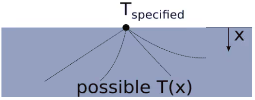For the constant temperature boundary condition, the surface temperature is assumed to remain at the specified value. Regardless of how much heat passes through the surface.  

In general, the specified surface temperature can change with time, and can also be different for distinct points on the boundary.  Physically, constant temperature boundary conditions are often approximated very well by phase change (boiling, melting, condensation, etc.) at the surface.  

The energy associated with phase change absorbs or supplies large amounts of heat at the phase change temperature.

Constant Heat Flux Conditions

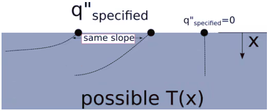For the constant heat flux case, the heat flux at the surface is assumed to remain at the specified value regardless of what happens to the temperature.  Again, in the most general case, the specified heat flux can be a function of time and position.  

Over a limited range of temperatures, a constant heat flux boundary condition might be approximated by a thin electrical resistance heater, or by radiative heating from a source that is at a much, much higher temperature than the surface.  A well-insulated surface constitutes a special case of a constant heat flux boundary condition where the heat flux is specified as zero.  This is called an adiabatic surface.

Convection Boundary Conditions

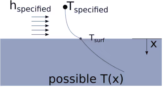A convection boundary condition occurs when the surface is exposed to convective heat transfer governed by Newton’s law of cooling.  The convective heat transfer coefficient and the free stream temperature could, in general, both be functions of time and position.

A simple example of one-dimensional, steady-state heat transfer can illustrate the effect and application of different boundary conditions.  The governing differential equation (assuming constant properties) is simply:

Which can be integrated twice to yield:

T (x) = A * x + B

Where A and B are constants of integration that will be determined by the boundary conditions.  The structure of the differential equation indicates that the temperature distribution will always be a straight line for this case, with a slope of “A” and a y-intercept of “B”.  Thus, the boundary conditions will determine the slope and the y-intercept of the temperature distribution.  

Constant temperature Boundary Conditions at Walls

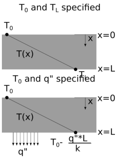
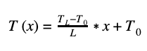
If we apply constant temperature boundary conditions at both walls: T(x=0)=T0, and T(x=L)=TL, then B=T0, and TL=A*L+T0, or A=(TL-T0)/L.  Putting these together, the temperature distribution in the wall is:

Now, let’s leave a constant temperature boundary condition at x=0: T(x=0)=T0, and apply a constant heat flux boundary condition at x=L: -k(dT/dx)|x=L = q’’ where it is assumed that the value of q’’ is specified.  The thermal conductivity of the body is “k”.  These boundary conditions result in the temperature distribution:

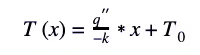
In the special case of the adiabatic wall, (q’’=0) the temperature distribution is just a constant, the imposed left side temperature, T0.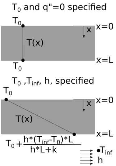

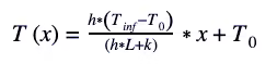
Finally, we address the constant temperature condition still on the left side. Here we can impose a convection condition on the right side : -k(dT/dx)|x=L = h*(T(x=L)-Tinf).  The temperature at x=L is A*L+T0, so the final temperature distribution is:

In real life, boundary conditions are rarely perfect, consistent, and completely known (as with material properties, geometry, surface conditions, etc.).  However, understanding the boundary conditions that went into the formulation of an equation or numerical model helps provide a realistic view of the assumptions and limitations of the model.

Biography

James Stevens is a professor in the mechanical and aerospace engineering department at the University of Colorado at Colorado Springs.  His background is in numerical and analytical heat transfer analysis. Covering both steady-state and transient situations with applications to thermal history, thermal response, electronic cooling, temperature profiles, thermal design, heat flow rate determination, and more. He also works in applied thermodynamics with applications for renewable energy, HVAC, air engines, novel heat engines, and more. He has over 30 years of experience in higher education teaching undergraduate and graduate classes. Performing research, doing course and curriculum development, and advising students.